In an earlier case study we took one AI-generated 5G LDPC decoder from 221 to 463 MHz, past a paid commercial IP on the same FPGA. That was a single configuration. The 5G LDPC standard supports two base graphs and 51 lifting factors, many code points in all. To show the timing method generalizes, we needed many more decoders, generated and tuned the same way.
Tuning one decoder by hand is not a design method. The real value of AI here is automating the process: generating and closing a batch of configurations, quickly, and proving every one correct, rather than tuning a single design.
Tuning one is the start; the tool is the goal
Every code point in the 5G LDPC standard maps to a different FPGA circuit. Change the configuration and the resource and timing work starts over. So instead of a person babysitting each one, we distilled the timing method into an automated flow: parameter-driven, it generates twenty decoders across configurations and closes timing and verifies correctness on each.
The twenty configurations cover both base graphs, two code rates each, and five lifting factors (Z = 32, 64, 128, 256, 384): base graph BG1 at rates 0.815 and 0.324, and BG2 at rates 0.588 and 0.192. Information lengths run from a few hundred to several thousand bits.
One skeleton, generated by parameters
This is the crux: the twenty decoders are not written twenty times by hand. They come from one generator, run with different parameters. The skeleton is the same folded layered decoder from the first case study (read estimate, run checks, accumulate and write back), where "folded" means processing a layer's hundreds of lanes in a few passes rather than all at once, saving a large amount of hardware while staying single-engine and zero-DSP.
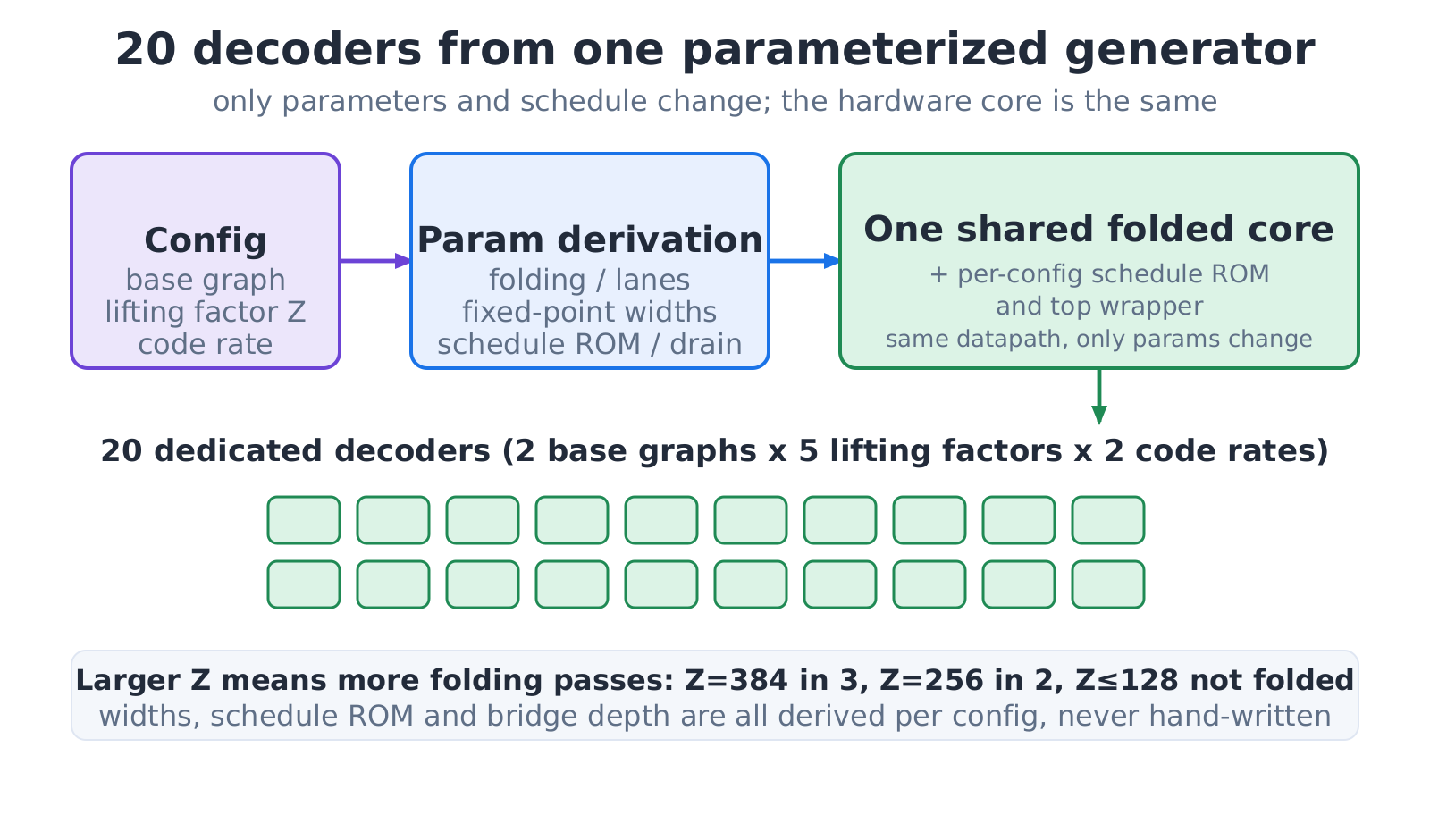
Given a configuration, the generator derives the fold count, the fixed-point widths, the schedule, and the stall cycles needed between layers, and emits a dedicated decoder. A larger lifting factor folds in more passes (Z=384 folds three ways, Z=256 two, 128 and below not at all); at smaller sizes the datapath itself narrows. None of this is set by hand. Twenty configurations, twenty parameter sets, that is all.
The risk in batch is batch-producing errors
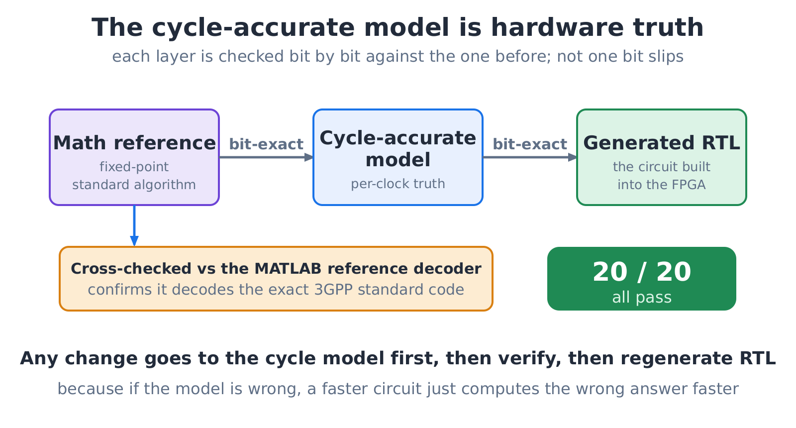
Generating fast is one thing; generating correct is another. A tool that produces quickly but produces errors is worse than nothing, so every decoder has to be proven correct first. There are three models, each closer to hardware: a mathematical reference of the standard algorithm, a cycle-accurate model, and finally the circuit synthesized into the FPGA. The rule is strict: any change goes into the cycle-accurate model first, is verified bit-for-bit, and only then regenerates the circuit. The cycle-accurate model is the hardware ground truth: if the model is wrong, faster hardware just computes the error faster.
Closure as a loop that rolls back
After a design is generated and verified, timing still has to be closed. In the first case study the cuts were found by hand, one at a time. Here that skill is rolled into a closed loop and pointed at all twenty configurations. For each design it first binary-searches how tight the clock target should be, then iterates a loop: measure across several placement strategies and take the median (a single run is noisy); locate the slowest path; select a fix from a library by the path's type; apply it, whether a constraint, a parameter, or a register in the middle of a long wire; then re-run the bit-exact and throughput checks; and accept if it got faster, or roll back and record the dead end so it is not tried again.
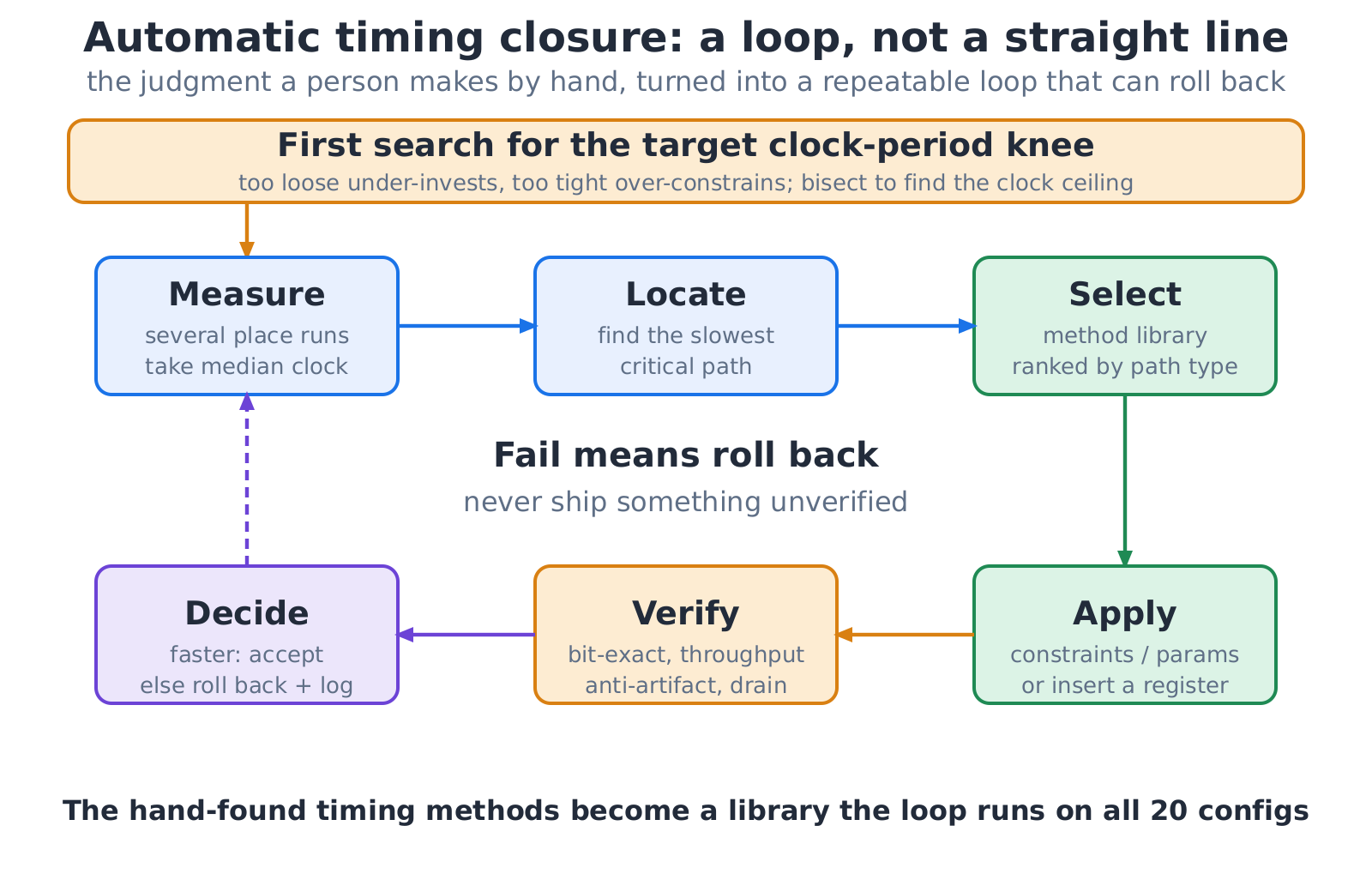
The most important property of this loop is that it rolls back. It would rather report "this point did not close" than hand over an unverified result as a success.
Results: clock matched, throughput close
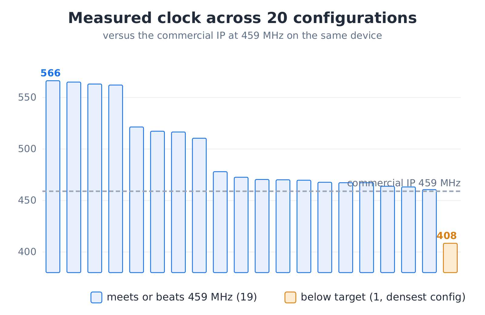
The flow generated, verified, and closed all twenty decoders. The device is the same FPGA the commercial IP names, at the same speed grade. Nineteen of the twenty matched or beat the IP's 459 MHz clock: a median of 1.03 times its clock, up to 566 MHz. The only one to miss was the densest configuration, held at 408 MHz by routing congestion; the tool reported it plainly, with nothing hidden.
Throughput, honestly
Throughput needs to be split out. The architecture is the same, so it should be close; the measured gap comes down to throughput techniques each side uses. Using the measured clock plus early stopping, eighteen of twenty beat the IP, but that lead comes from a higher clock and from terminating iterations early at good signal-to-noise, not from the architecture. Hold the clock and iteration count equal and compare codeword for codeword, and the IP leads again.
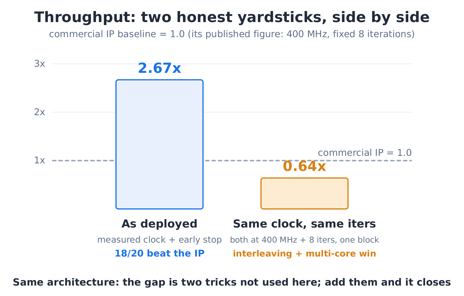
The difference is two throughput techniques this version does not use. One is block interleaving: because a layer must finish before the next begins, the pipeline waits a few cycles; the IP decodes several codewords interleaved, filling one codeword's wait with another's compute. The other is multiple check-node cores at small sizes: when the lifting factor is small the wide pipeline is underused, and the IP packs in several check-node cores to fill it, while our narrower datapath leaves the width idle. Both are addable; this version simply spends its budget on early stopping and a higher clock instead.
Why the tool matters more than one design
The first case study used AI to push one design past a commercial IP. This one used AI to build a flow that generates, closes, and bit-exact verifies twenty designs. The second is where AI compounds in hardware design. Accelerating one design is linear: one tuned, one earned. A tool is multiplicative: the same generator, the same verification net, the same closure loop, spread over more configurations, lowers the marginal cost of each.
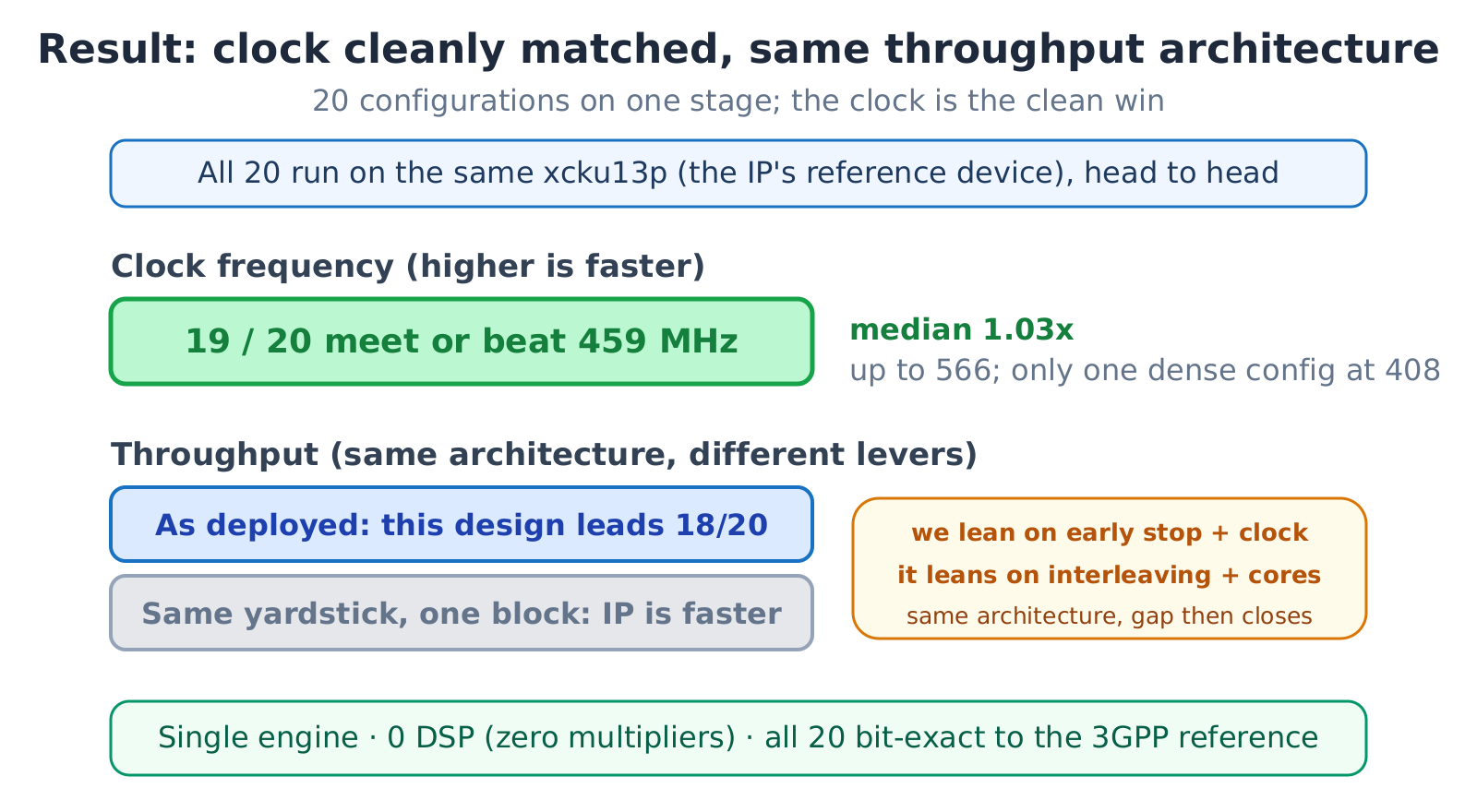
Twenty 5G LDPC decoders, one flow, nineteen matching or beating a paid IP's clock, every one matching the 3GPP reference bit for bit. That win belongs to the tool that produced them all, not to any single design.