1. The problem and the algorithm
A quantum error-correcting code is decoded every measurement cycle: the hardware reads a syndrome (which checks fired) and must infer the most likely set of errors fast enough that the backlog never grows. For superconducting qubits that budget is on the order of a microsecond per round, so the decoder is a hard real-time classical machine, not an offline solver.
Plain belief propagation, the workhorse of classical LDPC decoding, stalls on quantum codes: the stabilizer structure creates symmetric trapping sets where beliefs oscillate and never settle. Relay-BP (IBM's "Relay-ensembling with locally-averaged memory") adds three ideas that break that symmetry.
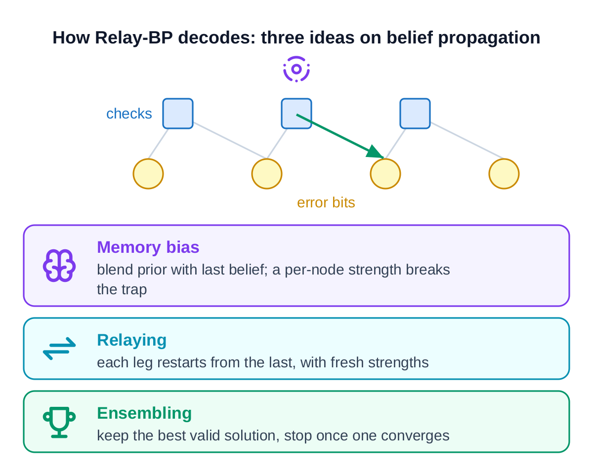
The memory bias blends each variable's prior with its previous belief by a per-node strength that may be negative; relaying carries beliefs from one leg to the next while redrawing those strengths; ensembling keeps the lowest-weight valid solution and stops once one converges. Empirically this beats general-purpose post-processing decoders by about an order of magnitude in logical error rate on the gross code [IBM, arXiv:2506.01779].
2. The hardware architecture
The reference silicon decoder is fully parallel: one compute unit per graph node and one wire per edge, so an entire belief-propagation iteration completes in two clock cycles. There is no central message memory; the messages live in the wiring fabric itself.
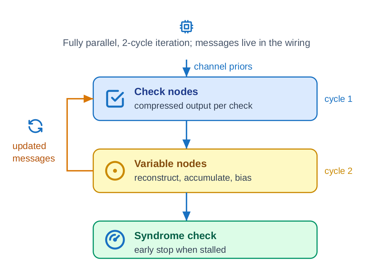
Two encodings keep that wiring affordable. Messages are carried in sign-magnitude form, so the magnitude is free of a sign bit on every edge. And each check node emits a compressed output (a sign, a selector, and the two smallest magnitudes) rather than a value per edge; the per-edge exclusive minimum is finished inside the variable node. Both shrink the bus that dominates the design.
3. The four compute units, up close
Everything that follows (the wiring ceiling, the lever map, the early-termination win) is a property of four small units repeated across the graph. This section is the foundation: each unit is shown at the datapath level, exactly as it is generated, so the later analysis can point back to a concrete circuit rather than a metaphor.
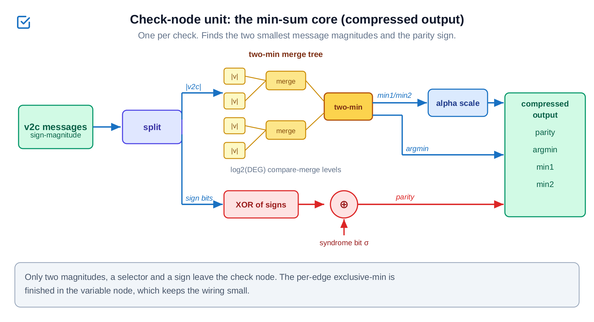
3.1 Check-node unit: the min-sum core
One per check. It splits each incoming sign-magnitude message, feeds the magnitudes into a two-minimum merge tree that finds the smallest and second-smallest plus the index of the smallest, and XORs the signs (against the measured syndrome bit) to a parity. Only that compressed tuple (parity, selector, two magnitudes) leaves the node. The exclusive-minimum-per-edge is deliberately not finished here; deferring it is what keeps the output bus narrow, and it is the single biggest reason the wiring stays affordable.
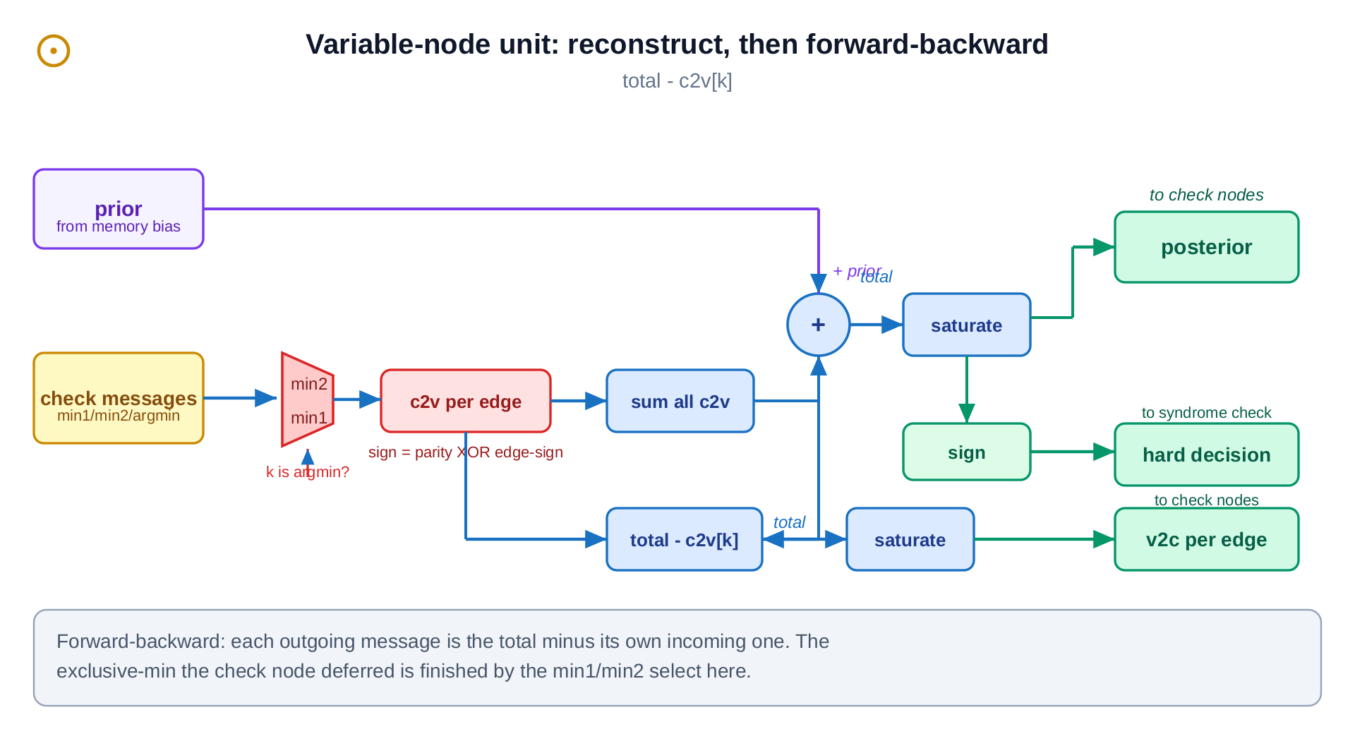
3.2 Variable-node unit: reconstruct and update
One per error bit. It reconstructs each check-to-variable message from the compressed tuple (picking the second-smallest magnitude when this edge is the selected minimum and the smallest otherwise, with the sign rebuilt from the parity), then sums all incoming messages with the prior, saturates, and emits a forward-backward update per edge (total minus this edge) plus a hard decision. The reconstruct MUX is the piece that pays back the check node's compression.
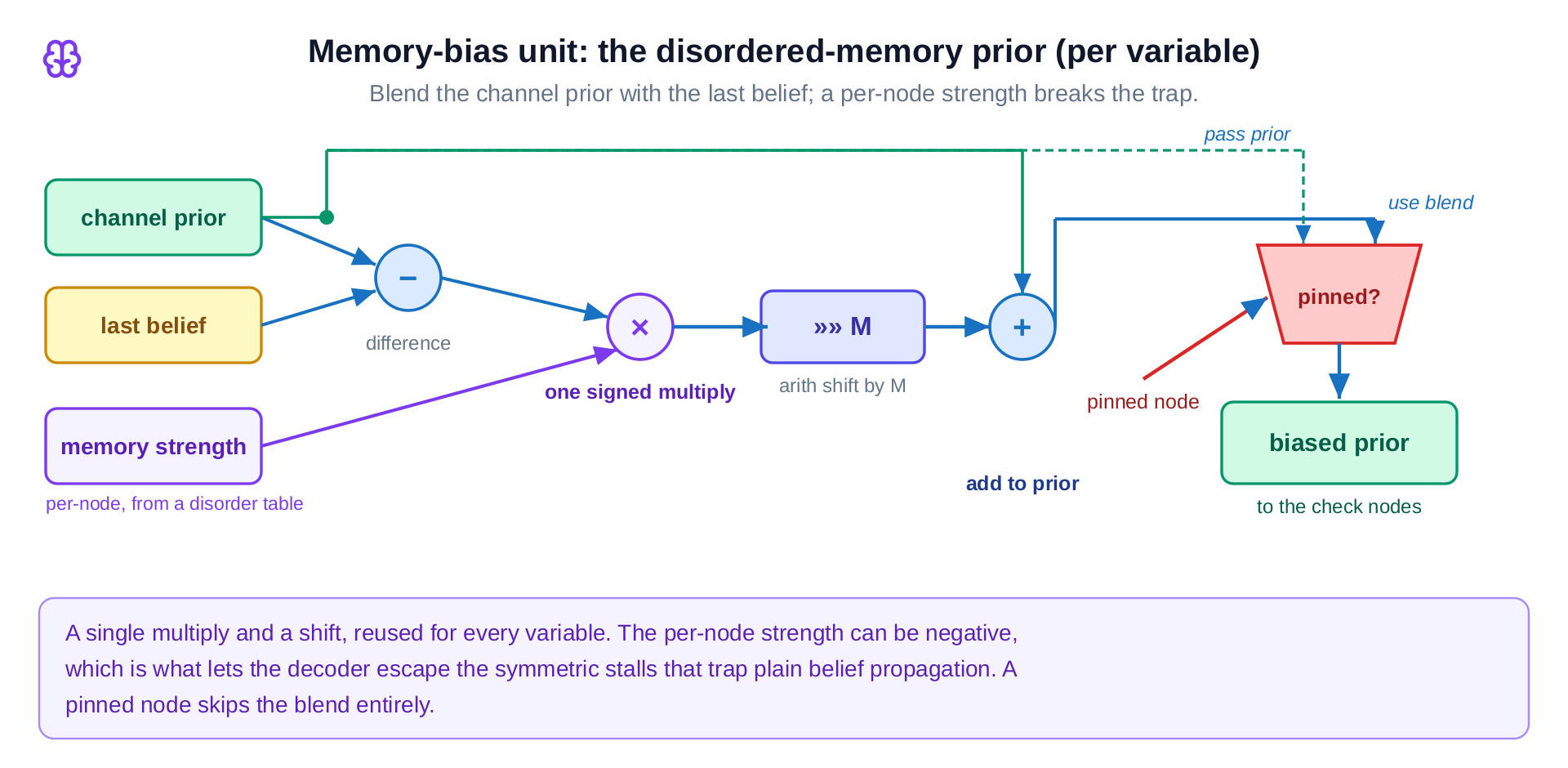
3.3 Memory-bias unit: the disordered-memory prior
This is the Relay-BP innovation, one instance per variable. It blends the channel prior with the last belief through a single signed multiply and an arithmetic shift (prior + strength × (belief − prior) >> M), and a pinned node passes its prior straight through. The per-node strength can be negative; that is precisely what lets the decoder escape the symmetric stalls that trap plain belief propagation, and it is why §1's "memory bias" is cheap in hardware.
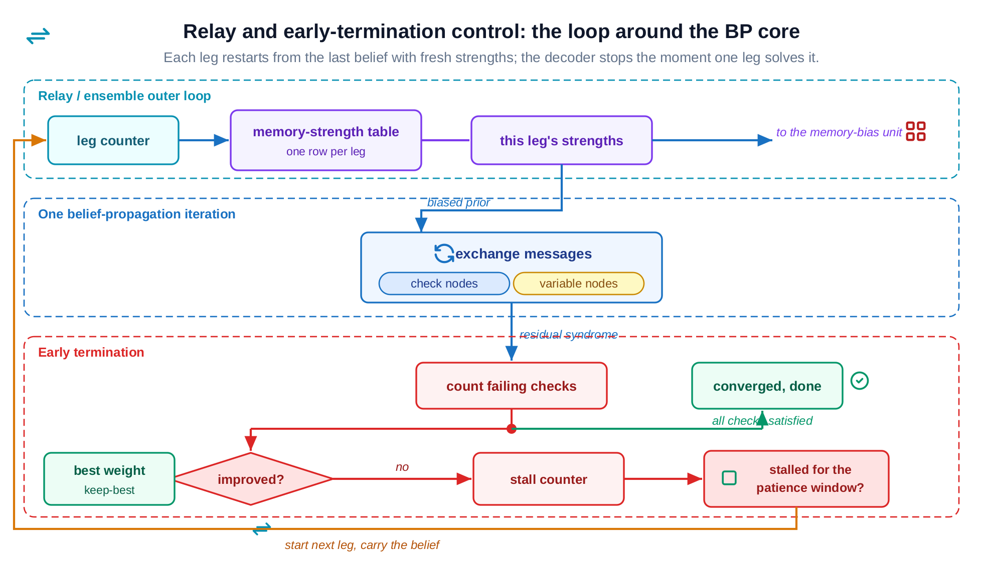
3.4 Relay and early-termination control: the outer loop
The control wraps the BP core. A leg counter indexes a memory-strength table (one row of per-node strengths per leg) that feeds the memory-bias unit; the belief carries forward from one leg to the next. A syndrome popcount counts the failing checks and drives two registers: a keep-best register that remembers the lowest-weight attempt (the ensembling), and a stall counter that ends a leg the moment progress stops for a patience window (the early termination). A cleared syndrome ends decoding immediately. This unit is where the optimization in §5 lives: the latency lever is the stall path drawn here.
4. Results and the wiring ceiling
Measured on the mid-scale distance-5 problem (a synthesizable proxy for the gross code) and compared against the published gross-code silicon:
| Configuration | LUT | FF | Clock | Provenance |
|---|---|---|---|---|
| This work, distance-5, fully parallel | 476,318 | 105,457 | ~85.7 MHz | MEASURED post-route, place-directive median |
| This work, gross extrapolation | ~2.2M | - | - | ESTIMATE linear scale from distance-5 |
| Published reference, gross, in silicon | 2,106,738 | 540,767 | ~83 MHz | arXiv:2510.21600 (XCVU19P, 58 W, 24 ns/iter) |
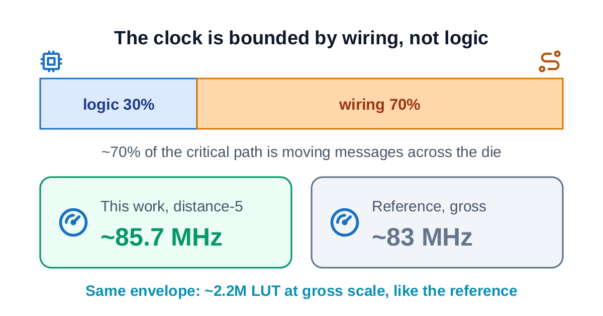
The clock is bounded by wiring, not logic: roughly 70% of the critical path is route delay across the die, an intrinsic property of the expander-style code graph. That is why the result matches the reference envelope rather than beating it: the wiring is the wall, and it is the same wall for everyone building this fully-parallel.
5. The optimization: real levers vs dead ends
Decode latency is iterations multiplied by cycles-per-iteration, divided by clock. With the clock pinned by routing, the honest map of what moved latency is short, and several intuitive levers actively hurt.
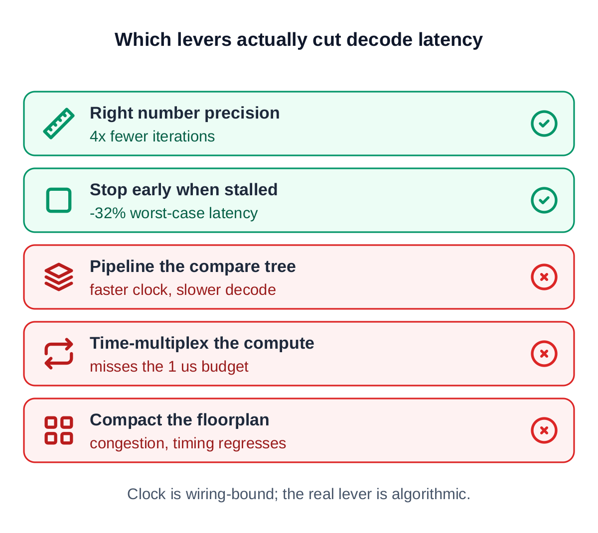
Choosing the right number precision cut iterations to a quarter (a smaller width converged far slower, so its area saving was a latency trap). Pipelining the comparison tree raised the clock but added a cycle per iteration, making per-decode latency worse. Time-multiplexing the compute could not meet the microsecond budget. Floorplanning the layout into fewer die regions traded crossing delay for congestion and regressed timing.
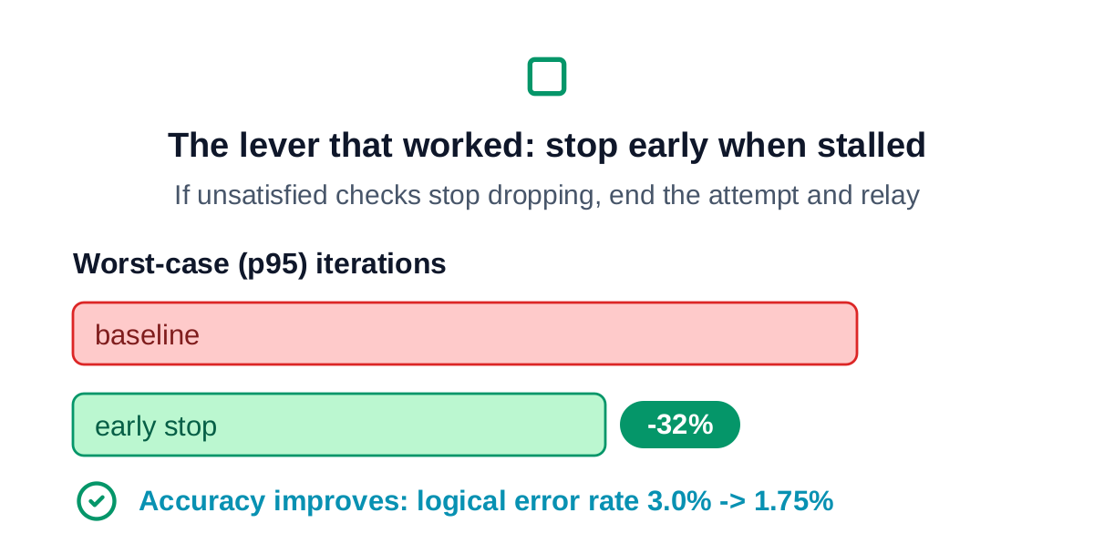
The lever that worked is algorithmic: end an attempt as soon as it stops making progress.
6. How correctness was assured
Every layer is held to the one below by bit-exact equality, so an optimization can never silently change the math.
- Math reference → cycle-accurate model → RTL. The math model is validated against the independent reference; the cycle-accurate model is validated against the math; the RTL is checked cycle-for-cycle against the model. All algorithm changes are made in the model first, then translated.
- Measure, do not compute. Pipeline depths and iteration counts are read from simulation, never estimated, because estimates were repeatedly wrong by a few cycles in ways that corrupt convergence.
- Hardest input first. Low-precision and convergence claims are tested on the hardest realistic inputs, not the easy all-zero case that hides sign and saturation bugs.
- Negative results are first-class. A fully-parallel gross build is not synthesizable on a generic flow; that was recorded, not hidden, and motivated the time-multiplexed path reserved for that scale.
7. Guidelines that transfer
- On a wiring-bound design, the clock is a property of the graph, not the logic; spend effort on fewer iterations or fewer wires, not on pipelining or floorplanning.
- Lower precision is only a win if it does not cost iterations; validate the iteration count, not just the area.
- Clock and per-decode latency are different objectives. A change that raises the clock can make latency worse if it adds a cycle per iteration.
- Validate any early-stopping policy on logical error rate at scale, not just convergence: the effect is subtle and can go either way.
8. Conclusion
The decoder, generated from a model proven equal to the math at every layer, sits on the published silicon envelope for the gross code: same clock regime, same resource scale. It is not faster because the wall is the code graph's wiring, which is the same for any fully-parallel implementation. The transferable contribution is the early-termination lever, a measured ~32% cut in worst-case latency at almost no area cost, validated to improve rather than degrade accuracy. Beyond this point, the levers are algorithmic (fewer iterations) or platform-level (a looser latency budget unlocking time-multiplexed area savings), not RTL tuning.